You submit the job, the solver runs, and somewhere in the middle it stops. The log has residuals and increment counts, but figuring out what actually went wrong, and where to look first, takes knowing how a problem solver works through your model step by step.

TLDR:

• A solver processes your fully configured model, mesh, boundary conditions, and loads, then solves [K]{u} = {f} to produce a converged output.

• Most convergence failures originate in pre-processing: bad contact definitions, under-constrained models, or load increments too large to track a load path.

• Direct solvers suit models under ~100,000 DOF; iterative solvers manage memory better for large, sparse systems but stall on poorly conditioned matrices.

• Your residual plot tells you where the job broke down: monotonically growing residuals point to setup, reversing residuals point to step size or material instability.

• Argus reads failed solver logs and proposes fixes you approve.

What a Solver Actually Is in Engineering Simulation

In engineering simulation, a solver is the numerical computation engine that takes your fully configured model and produces a solution. Geometry, mesh, boundary conditions, material properties, load steps: the solver receives all of that as input and works through the underlying system of equations to produce a converged output.

It sits late in the workflow by design. Before the solver runs, someone has already made dozens of upstream decisions. The solver itself makes none of them. Its job is to process what it was given, converge on a result, or tell you it couldn't.

In finite element analysis, this typically means solving a system of the form [K]{u} = {f}, where [K] is the stiffness matrix, {f} is the force vector, and {u} is the displacement field you're solving for.

Where the Solver Sits in the Simulation Pipeline

The CFD simulation workflow runs preprocessing, solver, then post-processing. The same structure holds in FEA tools like Ansys, Abaqus, and COMSOL, where an AI agent can now sit alongside the pipeline.

Pre-processing is where every upstream decision lives: geometry import, mesh generation, material definitions, boundary conditions, contact pairs, and load steps. The solver receives all of this as a fully assembled problem. It works with what was handed to it, without negotiating the geometry or questioning the mesh. For a closer look at how that translation from physical problem to configured model works, see bridging physical problems to FEA.

Post-processing picks up after convergence. Stress distributions, displacement fields, temperature gradients, residuals: those outputs only exist because the solver finished. The solver's role is the middle leg, largely invisible until something goes wrong.

What the Solver Actually Does Step by Step

Once you submit a job, the solver assembles a global stiffness matrix from every element in the mesh. Each element contributes a local stiffness, and these feed into one system-level equation set. Constraints and loads are then applied as modifications to that assembled matrix.

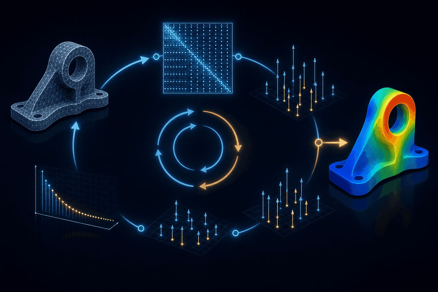
From there, the solver attempts to solve [K]{u} = {f}. Linear problems run in a single pass. Nonlinear problems break the load into increments, iterating within each one and updating the stiffness matrix as the solution evolves.

At every iteration, the solver computes residuals: the difference between internal forces and applied loads. If that residual falls below your convergence tolerance, the increment is accepted. If not, the job stops and logs why.

In CFD, the sequence runs over discretized governing equations, iterating across velocity, pressure, and scalar fields until residuals in each drop below threshold. The underlying logic is the same: guess, check, correct, repeat.

Direct Solvers vs. Iterative Solvers

Direct solvers invert the stiffness matrix, which makes them reliable and predictable but memory-hungry. For smaller models, that trade-off is fine. Once you cross into larger problem sizes, the memory overhead becomes a real constraint.

Iterative solvers approximate the solution through repeated refinement cycles, keeping memory usage manageable. The catch is that convergence depends heavily on preconditioner quality and how well-conditioned your problem is. A poorly conditioned matrix can cause an iterative solver to stall even when a direct solver would have pushed through, a pattern that shows up in compressible CFD simulations near transonic conditions.

Most commercial FEA tools choose automatically, but knowing which is running matters when a job fails or runs slower than expected.

How Mesh Quality Affects Solver Behavior

Mesh quality is one of the most direct levers over solver behavior, and it operates entirely upstream. By the time the solver runs, the damage from a bad mesh is already done.

Element shape metrics like aspect ratio, skewness, and Jacobian ratio aren't cosmetic concerns. Poor mesh shapes cause instability and divergence. A highly skewed element distorts the interpolation functions the solver relies on, and stretched elements with extreme aspect ratios produce ill-conditioned local stiffness matrices that erode convergence across the global system.

Mesh convergence studies quantify discretization error. Refining the mesh and checking whether the output stabilizes is how you separate solver noise from physics.

When a solver fails or produces suspect results, check the mesh first. Adjusting solver tolerances or switching algorithms treats the symptom. Degraded element quality is often the actual source.

Why Convergence Fails and What the Solver Is Telling You

Convergence failure is the solver telling you something specific. Reading it that way, instead of treating it as a run error to brute-force past, is what separates a quick fix from a half-day of re-runs.

The four failure modes that account for most diverged jobs:

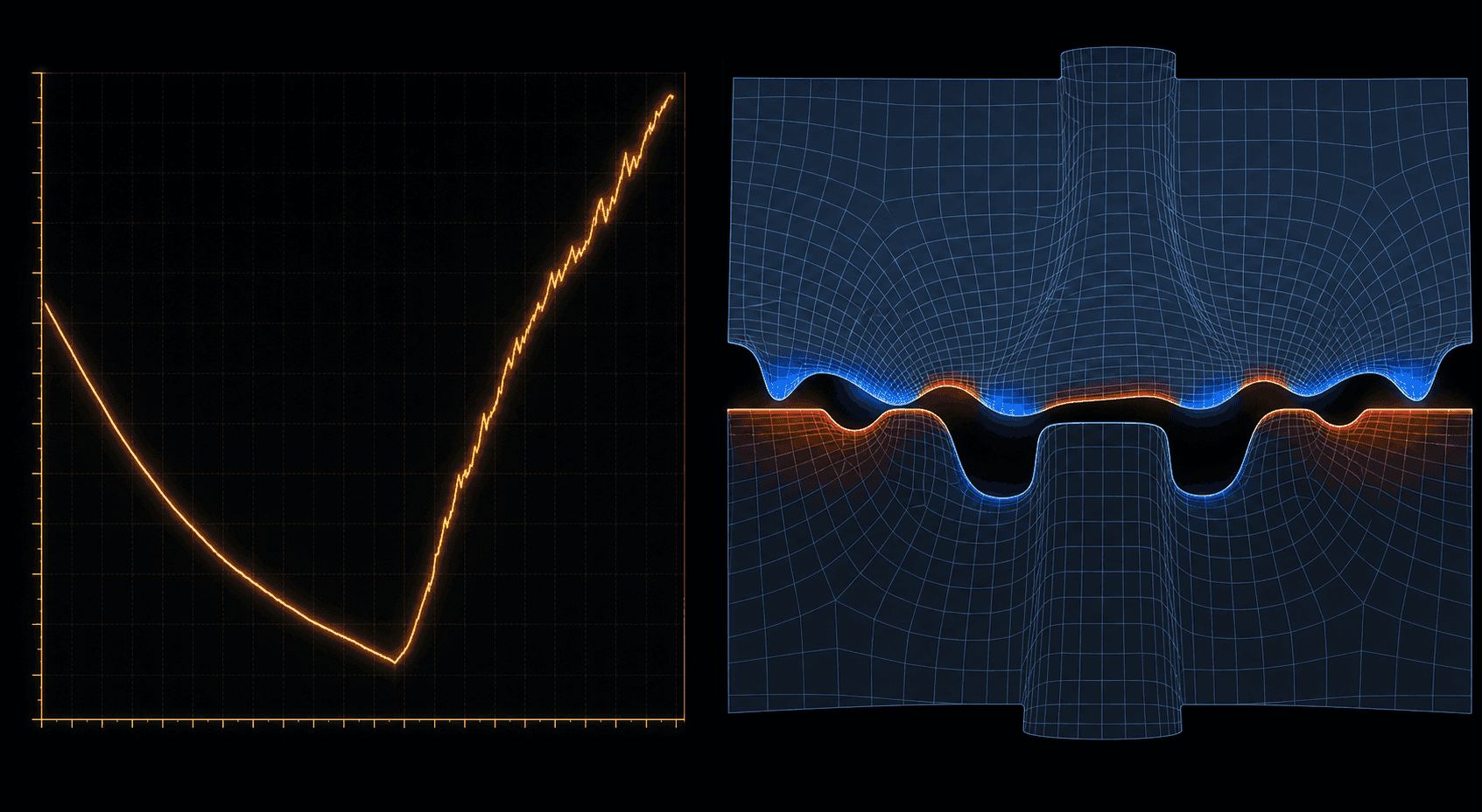
• Nonlinear material behavior pulling the Newton-Raphson iteration outside its convergence radius. If the tangent stiffness changes too sharply between iterations, the corrector overshoots and the residual grows instead of shrinking. Smaller load increments or a line-search method usually recovers it.

• Contact instabilities causing chattering, where nodes oscillate between open and closed status across iterations. The residual bounces without trending down. Stabilization parameters or adjusting the contact penalty stiffness typically settles it.

• Boundary condition misconfigurations producing under-constrained or over-constrained models. An under-constrained model produces rigid body motion; the solver sees unbounded displacements and the stiffness matrix becomes singular. Over-constraint locks competing conditions against each other and the residual never finds a physically consistent solution.

• Load increments too large for the solver to track a meaningful load path. The job skips over the equilibrium state entirely and diverges on the first iteration of that increment.

The residual plot is your first diagnostic. A residual that grows monotonically from the first iteration points to a setup problem, often contact or boundary conditions. One that decreases for several iterations then reverses usually signals a step size issue or a material instability entering at that load level. A flat residual that neither grows nor drops often means the solver is stuck at a saddle point in the solution space, and a perturbation to the initial conditions or contact formulation will get it moving again.

Nonlinear Solvers and Why They Are Different

Linear solvers solve the problem in one shot: the stiffness matrix goes in, the solution comes out. Nonlinear problems don't work that way because the stiffness itself changes as the solution evolves. That means you can't assemble [K] once and solve; the solver has to repeatedly update the stiffness, apply a correction, check the residual, and iterate until the solution balances again.

Large deformation, plasticity, hyperelastic materials, contact: in each case, the relationship between load and response depends on the current state of the model. You can't assemble [K] once and invert it. The solver has to track how [K] changes as deformation accumulates, breaking the total load into increments and iterating within each one.

Newton-Raphson and Its Limits

The Newton-Raphson method is the standard approach. At each increment, the solver computes a displacement correction based on the current residual and tangent stiffness, applies it, recomputes the residual, and repeats until the residual falls below tolerance. State variables like plastic strain or damage carry forward from one increment to the next and feed directly into how stiffness is recalculated.

When the load path hits a snap-through or structural instability, Newton-Raphson can fail because the tangent stiffness becomes singular near the limit point. Arc-length methods handle this by controlling load and displacement simultaneously, letting the solver trace around the instability and continue past it.

Sub-increments matter when material behavior changes sharply within a single load step. Finer sub-increments reduce linearization error across a highly nonlinear load path, at the cost of more iterations per step.

Solver Selection Trade-Offs Across Ansys, Abaqus, and COMSOL

Each tool surfaces solver choices differently, but the underlying trade-offs are consistent across the board.

Ansys Mechanical

Ansys defaults to the sparse direct solver for most structural analyses, which holds up well across a wide range of model sizes and contact configurations. The PCG (preconditioned conjugate gradient) iterative option becomes worth considering when model size pushes memory limits, particularly for large shell or beam assemblies. PCG convergence depends on how well-conditioned the system is, so models with poor mesh quality or numerically difficult contact tend to stall.

Abaqus

Abaqus also uses a sparse direct solver by default. The real choices surface in contact formulation: the penalty method is more computationally forgiving but introduces a compliance error proportional to the penalty stiffness, while the Lagrange multiplier approach is more exact but increases system size and can slow convergence in models with large sliding or complex contact topology.

COMSOL Multiphysics

COMSOL offers MUMPS and PARDISO as its primary direct solvers for coupled physics problems. For larger models, iterative solvers with geometric multigrid preconditioning can cut memory cost by a measurable margin. Multiphysics coupling often produces ill-conditioned systems, so iterative performance varies more here than in pure structural cases. See how an AI agent for COMSOL multiphysics can help manage that complexity.

How Upstream Configuration Decisions Drive Solver Outcomes

Most solver failures don't originate in the solver. They originate in pre-processing, and the solver is simply the first place that reports them.

Four configuration categories account for the majority of root causes:

• Contact definitions with incorrect formulation, missing pairs, or mismatched surface normals

• Boundary conditions that leave the model under-constrained, over-constrained, or physically inconsistent with the load sequence

• Material model parameters outside valid ranges for the expected strain or temperature regime

• Load step sequencing that jumps too aggressively or applies conditions in an order the physics can't support

Working backwards from a solver error is the more reliable diagnostic path. A singular stiffness matrix almost always points to rigid body motion from an under-constrained model. Oscillating residuals with no downward trend tend to mean contact is chattering, which leads back to penalty stiffness or surface pair definitions.

The solver log gives you the increment and iteration where the job stopped. That timestamp is your anchor. Go back to what changed in the model at that load level, and the configuration error is usually close.

Reading and Interpreting Solver Logs

Solver logs follow a consistent structure once you know what to look for.

Each iteration line typically reports the increment number, iteration count, and current residual norm for force and displacement. In Abaqus, these appear as force residual and displacement correction values checked against your convergence criteria. Ansys reports similar quantities alongside contact status changes per iteration.

A healthy convergence history shows residuals dropping roughly by an order of magnitude across successive iterations. Newton-Raphson converges quadratically when working: the residual collapses in the final iterations before acceptance. A steady, gradual decline without that late-stage acceleration suggests a modified tangent or mild nonlinearity.

Watch for these signals in the log:

• Residual norms increasing within a single increment: the corrector is overshooting.

• Increment bisection messages: the solver cut step size automatically because the previous size couldn't support convergence.

• Near-zero pivot or zero-energy mode warnings: the stiffness matrix is approaching singularity, usually from rigid body motion or a collapsed element.

• Contact status oscillating between open and closed across consecutive iterations: chattering, not convergence.

The increment where the job terminates is the most useful anchor. Cross-reference it with the load level applied at that point, then work back through the contact status and residual history from the prior increment. If that increment converged cleanly and this one diverged immediately, the issue likely triggered at a specific load threshold, pointing to a material instability or contact event at that state.

How Argus Approaches Solver Diagnostics and Pre-Simulation Setup

Argus works inside Ansys, Abaqus, COMSOL Multiphysics, Star-CCM+, and HyperMesh, handling pre-simulation configuration before a job ever runs. Boundary conditions, contact definitions, material parameters, load steps: Argus asks clarifying questions before committing any of it, then presents a complete model summary for engineer sign-off. Nothing executes until you approve it. When a run does fail, every action taken is logged, traceable, and reversible within your own tools.

For parametric work, Argus runs autonomous Design of Experiments sweeps across solver configurations or design variables, synthesizing results into comparative tables and flagging where returns diminish. Onboarding takes one to two hours across 15+ CAD/CAE/PLM tools, with no migration or new file formats required.

Final Thoughts on Solver Failures and the Decisions Behind Them

A diverged job is information. The residual history, the load level, the contact status across the last few iterations: taken together, they usually point to one specific setup decision that didn't hold. Your job is to read that signal, not adjust tolerances and resubmit blind. Argus surfaces that reasoning step by step and hands the fix back to you, inside the tools you already use.

FAQ

Why does my solver diverge even when the mesh looks clean?

Divergence most often traces back to pre-processing, not the solver itself. The four most common root causes are contact instability, under-constrained boundary conditions, material parameters outside valid ranges, and load increments too large to track the equilibrium path. Start with the residual plot and the increment where the job stopped, then work backwards through contact status and boundary conditions at that load level.

How do I read solver logs in Ansys and Abaqus to diagnose convergence failures faster?

Look at three things in sequence: whether residual norms are growing within a single increment (the corrector is overshooting), whether the solver issued increment bisection messages (step size was cut automatically), and whether contact status is oscillating between open and closed across iterations. In Abaqus, force residual and displacement correction values appear against your convergence criteria each iteration; in Ansys, contact status changes are logged per iteration alongside those quantities. The increment where the job stops is your anchor.

Direct solver vs. iterative solver in FEA: which should I use in Ansys or Abaqus?

For models under roughly 100,000 degrees of freedom, direct solvers like the sparse direct option in Ansys and Abaqus are reliable and predictable. For larger, memory-constrained problems, iterative options like PCG in Ansys or MUMPS/PARDISO in COMSOL become worth evaluating, but convergence depends on how well-conditioned your system is. A poorly conditioned matrix from degraded mesh quality or difficult contact can stall an iterative solver where a direct solver would have pushed through.

What are the best practices for prompting an AI agent to get better results on complex FEA or CFD setup tasks?

Give the agent the full context upfront: geometry state, intended physics, known constraints, and what the previous run produced if you are diagnosing a failure. Vague prompts produce generic responses; specific inputs like contact pair definitions, material regimes, and load step sequences let the agent reason from the actual model state. With Argus, the agent asks clarifying questions before committing any configuration and presents a full model summary for your sign-off before executing, so the prompt exchange itself becomes a structured setup review rather than a guess-and-check loop.

Where is engineering data stored when an AI agent runs solver diagnostics or pre-simulation setup?

With Argus deployed on-premises, CAD files, simulation inputs, and PLM records stay within your own infrastructure and are never ingested by Cosmon. When running in cloud mode, data is processed via Anthropic under a zero data retention contract, with an option to disable telemetry. Every action the agent takes is logged, traceable, and reversible within your own tools regardless of deployment model.